Sheets Import Range: How to Set Up and Fix It
The regional sales workbook sits in one tab. The dashboard sits in the next. You type =IMPORTRANGE, paste the link, hit Enter, and the cell answers with #REF!.
Or it works on day one and then dies in month four, on the morning of a review, when the source sheet has grown past what the formula can carry.
Either way, the fix usually isn't a different function. It's a better range. Google Sheets had approximately 1.1 billion users worldwide in 2025, according to ElectroIQ's Google Sheets statistics, which means an enormous number of files are linked to other files, often by people who learned the syntax in thirty seconds and never learned the rest.
Here's the whole picture, from the first paste to the checklist that tells you the import will still be running next quarter.
How to Write an IMPORTRANGE Formula
Start from the finished line, then take it apart. Paste this into an empty cell in the file that should receive the data:
=IMPORTRANGE("https://docs.google.com/spreadsheets/d/1AbCdEfGhIjK/edit", "Sheet1!A1:D500")
Two arguments sit between the parentheses, separated by a comma. The first argument is the source spreadsheet URL. Copy the full address from the browser address bar of the source file, paste it between double quotes, and leave nothing out. A partial link, or a link to a different file, won't connect.
The second argument is the range string, and it has two halves joined by an exclamation mark. The sheet name goes on the left of the exclamation mark, the cell block on the right, both inside double quotes.
| Argument | What to enter | Example |
|---|---|---|
| Spreadsheet URL | Full address of the source file in double quotes | "[source-file-URL]" |
| Bounded range | Sheet name and cell block in double quotes | "Sheet1!A1:D500" |
| Whole column | Sheet name and column letters only | "Sheet1!A:A" |
| Sheet name with spaces | Name wrapped in single quotes inside the range | "'Monthly Sales'!A1:C" |
Look at that last row. Any sheet name containing a space needs single quotes wrapped around it inside the double-quoted string. Drop them and the formula won't even parse, which is a different failure from a range that parses and returns nothing.
The spill rule nobody mentions first
The formula spills. Whatever sits below and to the right of the anchor cell has to stay empty, because the import needs that space for the values it brings in. One stray note three rows down and the cell throws #REF! even though the source, the link and the permission are all fine. Clear the spill path before you debug anything else.
Bounded range or whole column
If the source has a fixed number of rows, use a bounded range such as Sheet1!A1:D500. It transfers less data, it's easier to debug, and when the numbers look wrong you can compare the same visible block in both files. Reach for A:A only when the row count changes without warning and you can't predict where the data ends.
With the URL copied, the range correct and an empty cell chosen, you have a formula ready to paste. Everything after this point is permission.
How to Grant Access and Connect Two Files
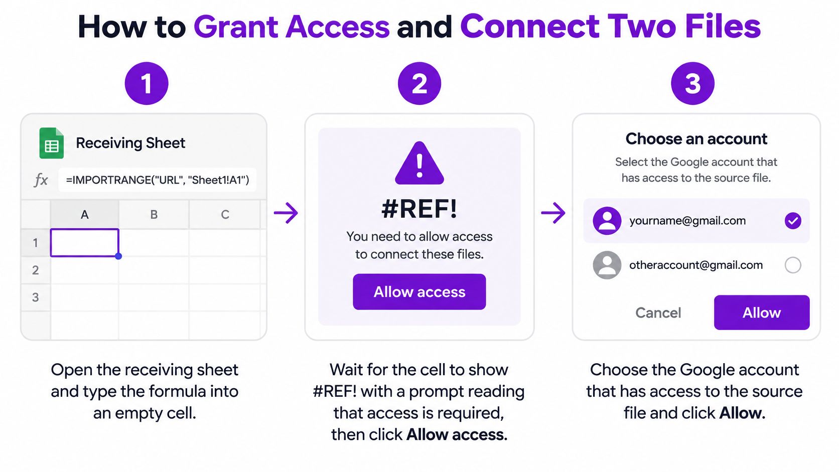
The first time you connect two files, Sheets won't read a single cell until you approve the link. Here's the routine, with the reason behind each step.
- Type the formula into an empty cell in the receiving file. The cell you choose is the anchor. Every value lands below and to the right of it, so pick a spot with room to grow.
- Wait for the #REF! and the prompt saying access is required. That error isn't a mistake in your formula. Google is telling you the two files have no connection yet, and it can't read across files without your consent.
- Click Allow access, then pick the Google account that can already view the source file. The grant is stored against an account, not against a browser or a device. Choose the account with view rights and values appear.
- Confirm values fill the cells below and to the right. This is your proof the range string matched something real. If the error clears but the grid stays empty, the sheet name or the cell block is wrong.
- If the prompt never appears, open the source file, click Share, and add the importing account with at least Viewer access. Waiting won't fix this one. Without view rights on the source, the prompt has nothing to resolve.
The grant happens once per pair of files, not once per formula. Ten IMPORTRANGE formulas between the same two workbooks need one approval, and the tenth doesn't ask again.
The most common slip: the browser is signed into a personal account while the source file belongs to a work account. The prompt appears, you click Allow, and the wrong identity gets recorded. Check the account avatar in the top right corner before you approve anything.
A working import looks like this: values filling the grid, the anchor cell holding a formula with no error, and the source file unchanged. Approving the connection doesn't alter sharing settings on either file, so you're not handing out access by accident.
Live Examples for Common Import Jobs
Three setups, three formulas, three design decisions. Copy whichever matches the job in front of you.

A budget tracker that shows the current month. A finance lead keeps the regional sales workbook separate from the team dashboard, and the dashboard only ever needs the current month block, which tops out around 200 rows.
=IMPORTRANGE("https://docs.google.com/spreadsheets/d/1RegionalSales/edit", "Current Month!A1:F200")
The decision: bounded, not A:F. The dashboard pulls six columns and a known number of rows instead of every stray annotation anyone ever typed in column H. When a figure looks wrong, you can open the source and compare the identical block.
An index built from a whole column. A hiring coordinator tracks applicants in one sheet and wants a list of company names in another, where new rows arrive every week.
=IMPORTRANGE("https://docs.google.com/spreadsheets/d/1JobTracker/edit", "Job Tracker!B:B")
The decision: whole column, because a bounded range would need editing the first time someone adds row 501. Pull the one column you need rather than A:Z, so the request stays small.
A filtered list that keeps its header. A job seeker wants only the rows where the status reads Applied, with the column names intact.
=QUERY(IMPORTRANGE("https://docs.google.com/spreadsheets/d/1Applications/edit", "Applications!A1:F2000"), "select * where Col5 = 'Applied'", 1)
The decision: the QUERY wrapper runs once in the anchor cell and filters the whole block on arrival. Don't place an IMPORTRANGE inside every row of a results column, because that becomes one request per cell. The closing 1 tells QUERY the source has a single header row.
A fourth pattern worth knowing. Two IMPORTRANGE formulas on separate tabs, each pulling from a different source, feeding a summary tab through plain cell references. Each pair of files keeps its own access grant, so revoking one connection leaves the other working.
If your source data starts life as a download rather than a shared file, the guide to importing a CSV into Google Sheets covers the step that comes before any of this.
Test any example the same way. Change one value in the source file, reopen the receiving file, and confirm the new value appears. If it doesn't, the problem is permission or the range, not the function.
Error Messages and How to Fix Them
Nearly every IMPORTRANGE complaint traces back to the same handful of causes, and they arrive in a predictable order. The access prompt leads by a wide margin.
| Symptom | Likely cause | Fix |
|---|---|---|
| #REF! asking for access | Importing account has not approved the connection | Click Allow access, or ask the owner to share the source file |
| #REF! invalid URL or range | Broken link, wrong sheet name or missing quotes | Re-copy the URL and check the sheet name spelling and quotes |
| Loading message that never finishes | Too many imports or a very large range | Narrow the range and reduce the number of import formulas |
| Data exceeds 10 MB | Requested range is too big for one import | Split the range into smaller blocks across several cells |
| Data looks out of date | Import has not refreshed since the source changed | Reopen the receiving file, or wait up to an hour while it stays open |
| Errors after chained imports | One file imports from another that imports from a third | Consolidate the data into a single source file |
Look at the cost column hidden in that table. Re-granting access and fixing a typo take seconds. Splitting a source file that has outgrown a single request takes an afternoon, and collapsing three chained imports into one file can take a week of persuading other people to change their workflow.
Stale numbers are usually not broken numbers
A value you edited two minutes ago may not have crossed over yet. The import refreshes when the receiving file opens, and then on its own schedule while it stays open. Reopen the file before you rewrite the formula.
Every later error in the sheet follows from the formula sitting in the anchor cell. Check that cell first.
The same failure modes show up under different names when the receiving file feeds a field operation instead of a dashboard. If imports are driving outreach lists, this guide to fixing canvassing data sync issues walks the campaign-side version of the same hunt.
Keep Large Imports Fast and Within Limits
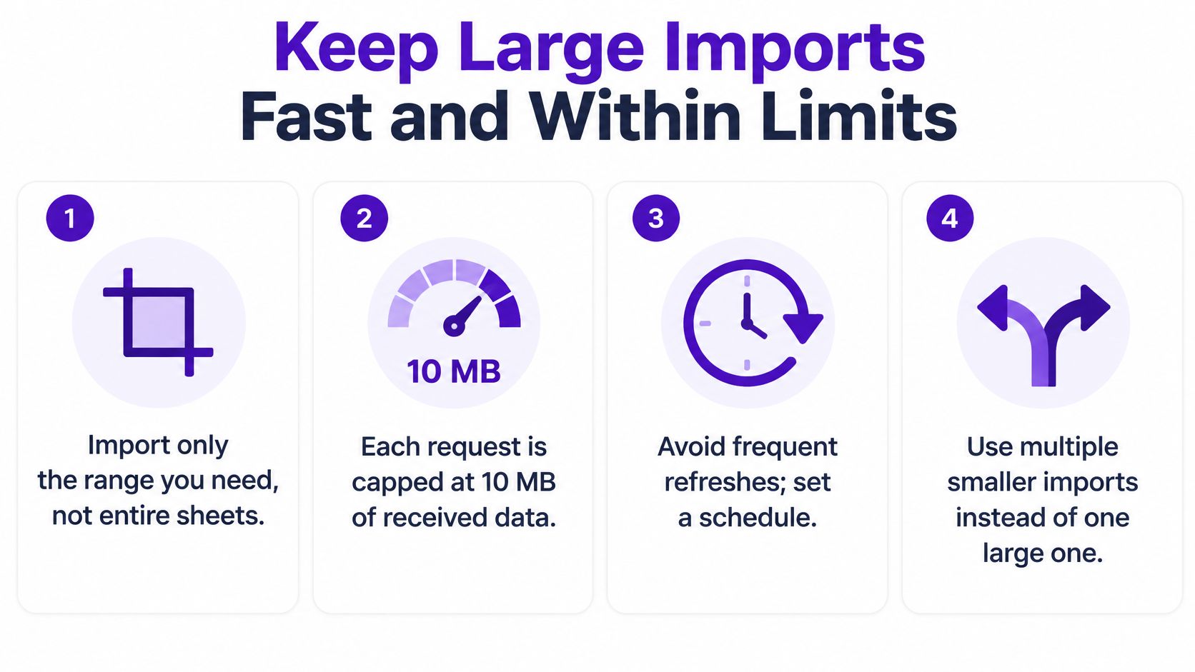
A common mental model is that IMPORTRANGE copies data once and stores it. It doesn't. Google's IMPORTRANGE documentation describes a live mechanism: Sheets downloads the entire requested range to your computer, each request is capped at 10 MB of received data, and the receiving file reloads imported data when it opens and checks for updates every hour while it stays open.
That's synchronization, not a copy, and it has a consequence the syntax tutorials skip. A source table that grows over months can break a formula that worked on day one, even though nobody touched the formula.
Rules that keep the import alive
- Bound the range to what you need. A worksheet area instead of an entire column cuts the data transferred on every refresh.
- Archive old rows in the source. Move last year's records to an archive tab. The live tab stays small and the import stays fast.
- Keep volatile formulas out of the same sheet. NOW, TODAY and RAND force recalculation, and recalculation pulls the import again.
- Pull once into a helper tab, then reference it. One import feeding a tab that other formulas read is cheaper than the same import repeated down a column.
- Avoid chains. A file importing from a file importing from a third is three points of failure for one number.
Google's guidance points the same way: frequent or numerous import functions can trigger loading or traffic-limit errors, so minimize volatile formulas, avoid excessive chained imports, and consolidate data where the option exists.
Rule of thumb: if an import takes more than a few seconds to load, shrink the range before you change anything else.
When IMPORTRANGE Is Not the Right Tool
Two ideas get mixed up here. A live link means the receiving file reads cells from another file each time it refreshes. A copy means the values are stored in the receiving file and stay put until someone updates them. IMPORTRANGE gives you a live link, and that's the right answer only when you want one.
| Method | Best for | Refresh | Setup effort |
|---|---|---|---|
| IMPORTRANGE | Live display of another file's cells | Reloads on open and checks hourly while open | Low, one access grant |
| Apps Script | Scheduled copies, transforms or writing to another file | Runs on a trigger you set | Medium, needs a script and a trigger |
| Paste as values | One-time snapshot that must stay fixed | None after the paste | Very low, no formula |
Apps Script suits a team that wants a fixed refresh time, say 6 a.m. before the morning standup, rather than open-and-hourly behavior. It also handles the jobs a formula can't touch, such as transforming rows on the way in or writing results back to another file. The price is a script and a trigger, plus someone who can maintain both.
Paste as values stops updating the moment you paste, which is exactly what you want when the source is an archive or a signed-off month that must never move.
A live link is a promise to maintain two files. A copy is a promise to maintain one.
The decision rule is short. Use IMPORTRANGE when the receiving file must show current data with no maintenance. Move to Apps Script when the job needs timing or needs to change the data. Paste as values when the snapshot itself is the point. And when the job is a one-time move rather than a permanent link, importing an existing spreadsheet removes the formula from the picture entirely.
Confirm Your Import Before You Rely on It
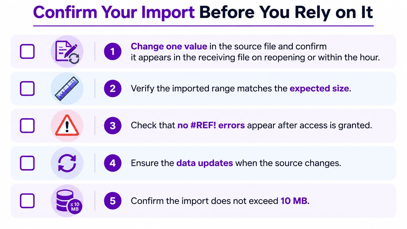
An import showing numbers today proves very little. Run these five checks before you build a decision on top of it.
- Change one value in the source. Reopen the receiving file and confirm the new value arrives, or wait for the refresh while it stays open.
- Confirm the importing account still has view access. People leave, folders move, and a grant that worked in January can stop working in April.
- Check the spill path. Nothing sits below or to the right of the anchor cell.
- Check the range is bounded and small enough for a single request.
- Check for chains. No file between these two imports from a third.
When all five pass, you can build on the number. If the data being imported is a job search log kept in a spreadsheet, Eztrackr takes the formulas out of the picture: you can import your existing jobs from a spreadsheet and let a board hold the records instead. The walkthrough on moving a spreadsheet-based job hunt into a tracker covers the format your rows need.
A job search tracked in a spreadsheet works right up until a formula breaks, and it always breaks on the morning you need the numbers. Eztrackr gives you a kanban board and a timeline that hold those records without a refresh schedule, and you can pull your existing rows across instead of retyping them. Head to Eztrackr and move your tracker off IMPORTRANGE for good.